Christoph M. Hoeppke


Vasicek interest rate model: analytic solutions, Monte Carlo approximations, and implementation trade-offs
Abstract
We study the Vasicek short-rate model and compare exact simulation with Euler-Maruyama approximation. We derive the analytic transition law, moment formulas, and zero-coupon bond price; then we test three simulation engines---pure loops, vectorized arrays, and JIT-compiled kernels---and benchmark them against closed-form reference values.Introduction
The Vasicek model (Vasicek, 1977) is the grandfather of short-rate models. Its spot rate $r(t)$ follows \[ dr(t) = a\bigl(b - r(t)\bigr)\,dt + \sigma\,dW(t), \qquad r(0) = r_0, \] with mean-reversion speed $a>0$, long-run mean $b$, volatility $\sigma>0$, and Brownian motion $W(t)$. The process is Gaussian, analytically tractable, and therefore a perfect laboratory for Monte Carlo: every simulated moment can be checked against an exact formula.We build three simulation engines around the same two schemes---exact sampling and Euler-Maruyama:
- a pure loop engine,
- a vectorized engine,
- a JIT-compiled engine.
Analytic solution of the Vasicek SDE
Deriving the transition law
Multiplying the SDE by the integrating factor $e^{at}$ gives \[ d\bigl(e^{at}r(t)\bigr) = a b e^{at}\,dt + \sigma e^{at}\,dW(t). \] Integrating from $s$ to $t$ ($s < t$) and multiplying by $e^{-at}$ yields the exact transition law \[ r(t) = r(s)e^{-a(t-s)} + b\bigl(1-e^{-a(t-s)}\bigr) + \sigma\int_s^t e^{-a(t-u)}\,dW(u). \]Proposition (Conditional distribution). Conditional on $\mathcal{F}_s$, $r(t)$ is normal with \[ \begin{align} \mathbb{E}\bigl[r(t)\mid \mathcal{F}_s\bigr] &= r(s)e^{-a(t-s)} + b\bigl(1-e^{-a(t-s)}\bigr), \\[4pt] \operatorname{Var}\bigl(r(t)\mid \mathcal{F}_s\bigr) &= \frac{\sigma^2}{2a}\bigl(1-e^{-2a(t-s)}\bigr). \end{align} \] Proof. The mean is zero because the stochastic integral has zero expectation. For the variance, It\^{o} isometry gives \[ \operatorname{Var}\bigl(r(t)\mid \mathcal{F}_s\bigr) = \sigma^2 \int_s^t e^{-2a(t-u)}\,du = \frac{\sigma^2}{2a}\bigl(1-e^{-2a(t-s)}\bigr). \] Setting $s=0$ gives the unconditional moments we use as benchmarks: \[ \begin{align} \mathbb{E}[r(t)] &= r_0 e^{-at} + b\bigl(1-e^{-at}\bigr), \\ \operatorname{Var}\bigl(r(t)\bigr) &= \frac{\sigma^2}{2a}\bigl(1-e^{-2at}\bigr). \end{align} \] Remark. As $t\to\infty$, $r(t)$ converges to $\mathcal{N}\bigl(b, \sigma^2/(2a)\bigr)$, the stationary OU distribution.
Exact versus Euler-Maruyama discretization
Exact discretization
Because the conditional law is Gaussian, we can sample the process exactly over a step $\Delta t = T/n_{\text{steps}}$: \[ r_{i+1} = r_i e^{-a\Delta t} + b\bigl(1-e^{-a\Delta t}\bigr) + \sqrt{\frac{\sigma^2}{2a}\bigl(1-e^{-2a\Delta t}\bigr)}\,Z. \]Euler-Maruyama approximation
The Euler scheme freezes drift and diffusion over $\Delta t$: \[ r_{i+1} = r_i + a\bigl(b-r_i\bigr)\Delta t + \sigma\sqrt{\Delta t}\,Z. \] It is first-order weakly consistent, but biased for finite $\Delta t$. The weak order of the Euler-Maruyama method is one under standard Lipschitz and growth conditions (Kloeden and Platen, 1992), so expectations of smooth path functionals converge at rate $\mathcal{O}(\Delta t)$. For the Vasicek model, the variance estimate is the most sensitive quantity because the scheme freezes the diffusion term at the start of each step (Higham, 2001).Comparison
The exact scheme has no discretization bias and cannot produce negative variances. The Euler scheme is simpler but visibly biased on coarse grids (Kloeden and Platen, 1992; Glasserman, 2004). Our convergence test confirms that the exact mean error never exceeds the Euler mean error for the same number of paths.Monte Carlo estimators
Moment estimation
From $N$ simulated paths we estimate \[ \hat{\mu}_N = \frac{1}{N}\sum_{j=1}^N r^{(j)}_T, \qquad \hat{\sigma}^2_N = \frac{1}{N}\sum_{j=1}^N \bigl(r^{(j)}_T - \hat{\mu}_N\bigr)^2. \] These converge almost surely to the analytic moments, with Monte Carlo error scaling as $1/\sqrt{N}$. In our convergence experiments we fix $N=10{,}000$ (normal) or $N=200{,}000$ (high) and measure \[ \epsilon_\mu = \bigl|\hat{\mu}_N - \mu\bigr|, \qquad \epsilon_{\sigma^2} = \bigl|\hat{\sigma}^2_N - \sigma^2\bigr|. \] Residual error is discretization bias for Euler (Kloeden and Platen, 1992) and pure Monte Carlo noise for exact.Zero-coupon bond pricing
The zero-coupon bond price is \[ P(0,T) = \mathbb{E}\left[\exp\left(-\int_0^T r(s)\,ds\right)\right]. \] Under Vasicek this is affine: \[ P(0,T) = A(0,T)\,e^{-B(0,T)r_0}, \] with \[ \begin{align} B(0,T) &= \frac{1-e^{-aT}}{a}, \\ A(0,T) &= \exp\left(\frac{\bigl(B(0,T)-T\bigr)(a^2b-\sigma^2/2)}{a^2} - \frac{\sigma^2 B(0,T)^2}{4a}\right). \end{align} \] We approximate the integral by the trapezoidal rule along each path and estimate the price by averaging discounted exponentials. The Monte Carlo estimate converges to the closed-form value as $N$ grows.Implementation strategies
Overview
We implement the same two schemes in three different ways. The choice is about where the loop lives and how much work is pushed from the interpreter into compiled code.Pure loop engine
The direct transcription uses nested loops and draws one standard normal per step. It is crystal clear, but every iteration pays interpreter overhead.
dt = T / n_steps
paths = [[0.0]*n_steps for _ in range(N)]
for j in range(N):
    r = r0
    for i in range(n_steps):
        z = random.gauss(0.0, 1.0)
        r = r + a*(b - r)*dt + sigma*sqrt(dt)*z
        paths[j][i] = r
return paths
Vectorized engine
We store the full $N \times n_{\text{steps}}$ path array and update all paths at once. Vectorization moves the arithmetic into compiled C kernels, but memory footprint grows with $N$.
dt = T / n_steps
paths = zeros((N, n_steps))
r = full(N, r0)
for i in range(n_steps):
    z = random_normal(size=N)
    r = r + a*(b - r)*dt + sigma*sqrt(dt)*z
    paths[:, i] = r
return paths
JIT-compiled engine
We keep the loop structure but compile the kernel to machine code. We pay a one-time compilation cost and then get cache-friendly, near-C speed.
@njit(cache=True)
def _simulate(r0, a, b, sigma, dt, n_steps, N):
    paths = zeros((N, n_steps))
    for j in range(N):
        r = r0
        for i in range(n_steps):
            z = random_normal()
            r = r + a*(b - r)*dt + sigma*sqrt(dt)*z
            paths[j, i] = r
    return paths

return _simulate(r0, a, b, sigma, dt, n_steps, N)
Observed performance trade-offs
Table 1 reports generation time for $N$ paths with $n_{\text{steps}}=50$.| $N$ paths | Pure (s) | Vectorized (s) | JIT (s) | Vec/Pure | JIT/Pure |
|---|---|---|---|---|---|
| 10,000 | 0.149 | 0.008 | 0.368 | 19.7$\times$ | 0.4$\times$ |
| 40,000 | 0.596 | 0.030 | 0.023 | 19.8$\times$ | 26.3$\times$ |
| 80,000 | 1.272 | 0.065 | 0.058 | 19.5$\times$ | 21.8$\times$ |
| 160,000 | 2.681 | 0.158 | 0.144 | 16.9$\times$ | 18.7$\times$ |
Table 1. Path generation times and speedups for our three engines. Parameters: $r_0=0.05$, $a=0.3$, $b=0.04$, $\sigma=0.015$, $T=2.0$, $50$ steps.
The JIT time at $N=10{,}000$ is dominated by compilation; once the cache is warm it is the fastest engine for large workloads. Both vectorized and JIT engines comfortably outperform the pure loop engine at production scale.
Numerical results and interpretation
Our experiments use \[ r_0 = 0.05,\quad a = 0.3,\quad b = 0.04,\quad \sigma = 0.015,\quad T = 2.0. \] The unconditional mean decays from $0.05$ toward $0.04$, and the long-run standard deviation is $\sigma/\sqrt{2a}\approx 0.0194$.Simulated paths
Figure 1 shows 100 exact paths with the analytic mean and 95% band.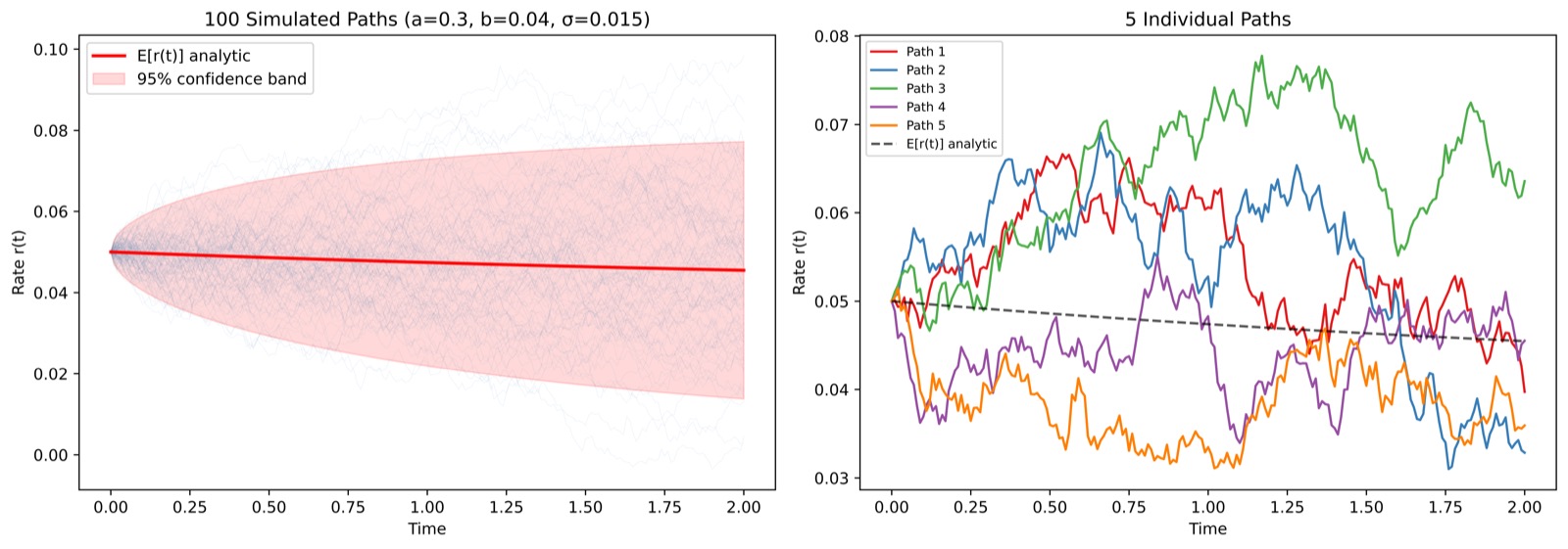
Figure 1. Left: 100 simulated paths with analytic mean and 95% band. Right: five individual trajectories.
Density at selected maturities
Figure 2 compares histograms of simulated $r(t)$ at $t=0.25,0.5,1.0,2.0$ with the analytic normal density.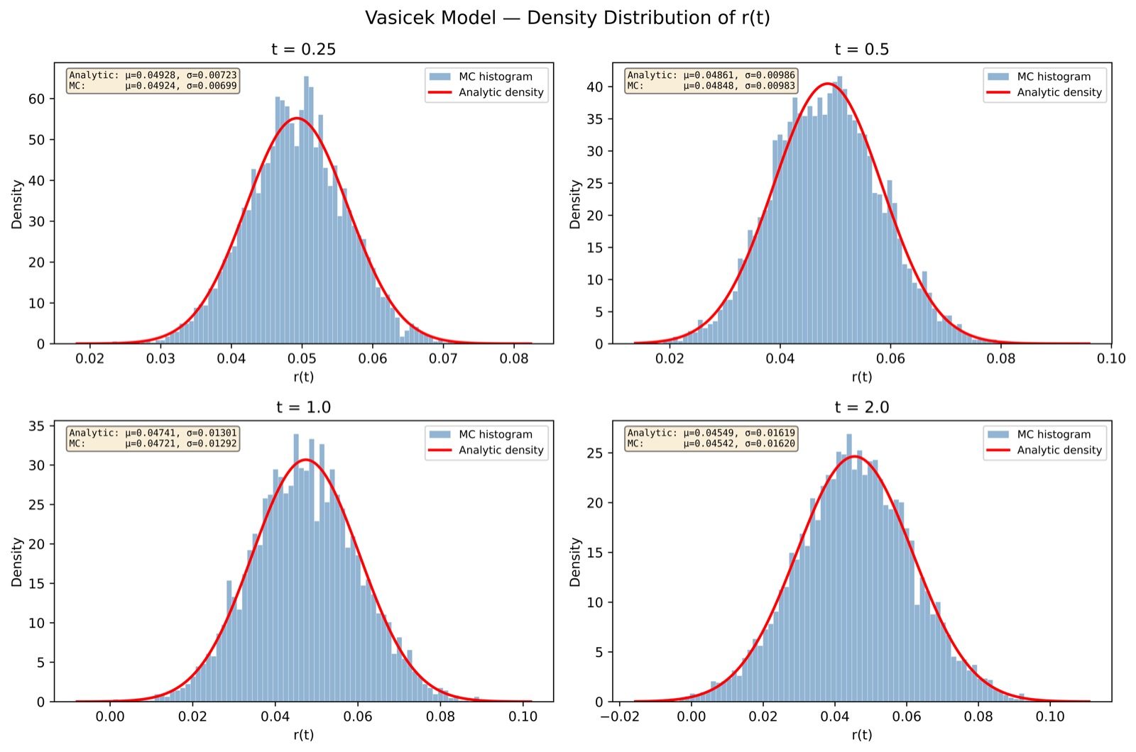
Figure 2. Histograms of simulated $r(t)$ versus the analytic normal density at selected horizons.
Convergence of mean and variance
Figure 3 plots absolute error in MC mean and variance against the number of time steps.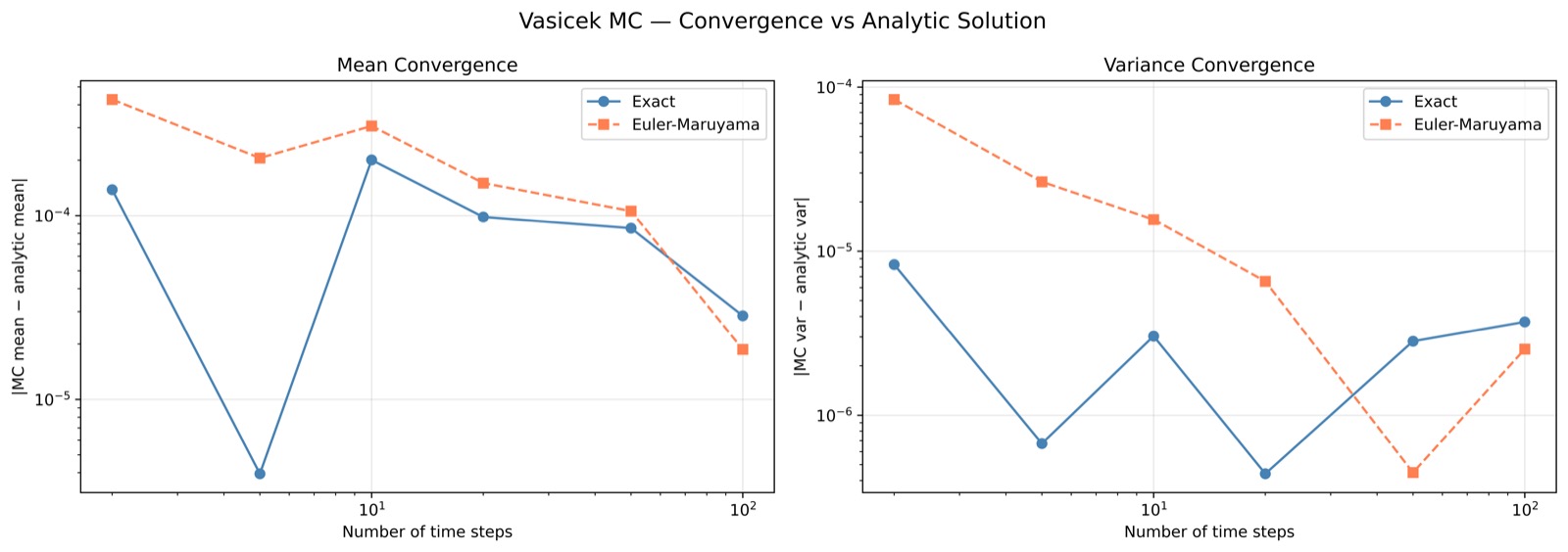
Figure 3. Convergence of MC mean and variance for exact and Euler-Maruyama schemes.
Speed of exact versus Euler schemes
Figure 4 benchmarks throughput of the two schemes in the JIT engine.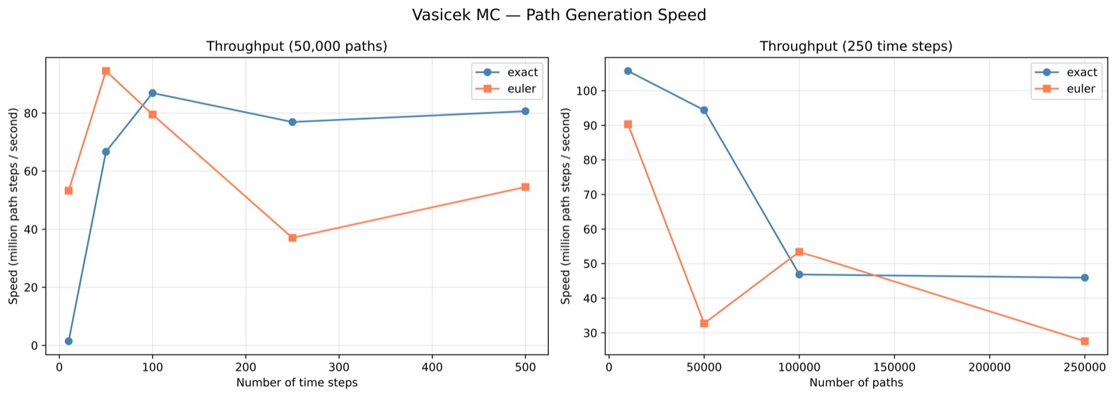
Figure 4. Path generation throughput for exact and Euler schemes across step counts and path counts.
Engine comparison
Figure 5 visualizes the timing results from Table 1.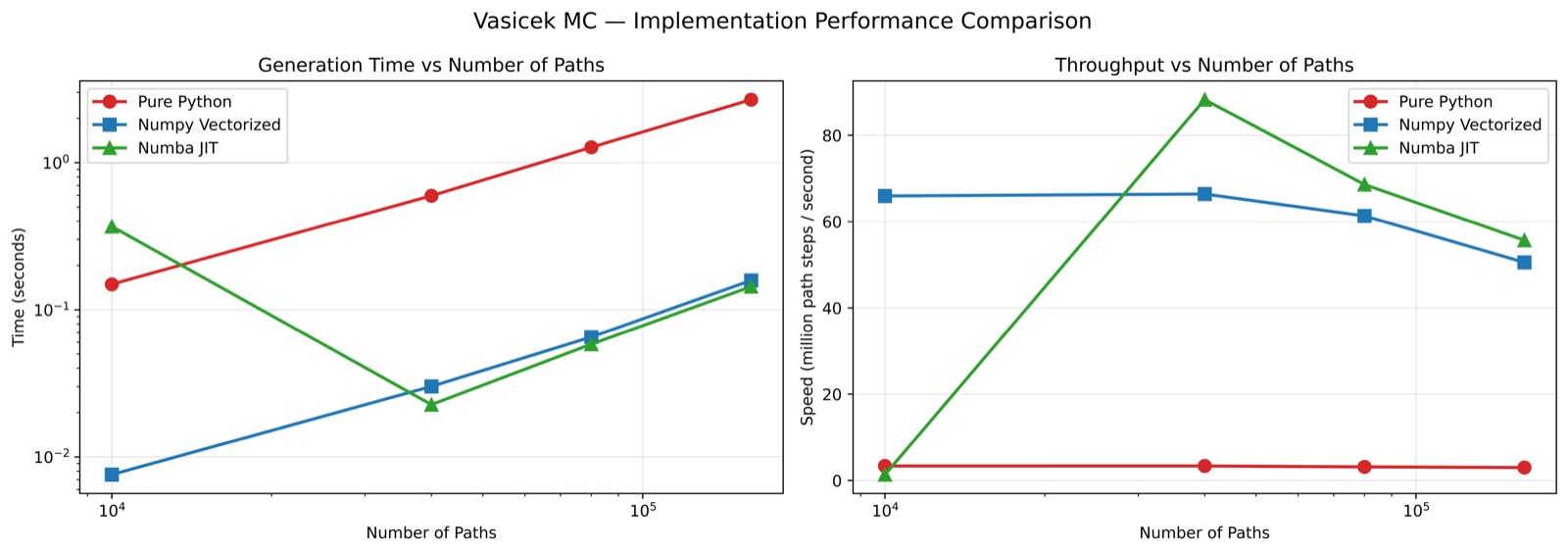
Figure 5. Left: generation time versus $N$. Right: throughput in millions of path steps per second.
Zero-coupon bond convergence
Figure 6 shows the Monte Carlo bond price converging to $P(0,2)\approx 0.909515$.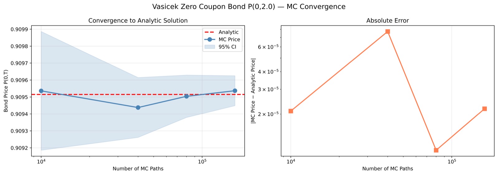
Figure 6. Left: MC bond price and 95% band versus the analytic price. Right: absolute error versus $N$.
Summary
- Exact simulation wins. The Gaussian transition law removes time-discretization bias; it is our default for Monte Carlo work.
- Euler is a useful benchmark. Simple and convergent, but biased on coarse grids.
- Engine choice dominates speed. Pure loops are correct but slow; vectorized and JIT engines give one to two orders of magnitude speedup. JIT is fastest once warm.
- Closed forms keep us honest. Analytic mean, variance, and bond price let us measure convergence without guesswork.
References
- Vasicek, O. (1977). An equilibrium characterization of the term structure. Journal of Financial Economics, 5(2), 177-188.
- Kloeden, P. E., and Platen, E. (1992). Numerical Solution of Stochastic Differential Equations. Springer.
- Higham, D. J. (2001). An algorithmic introduction to numerical simulation of stochastic differential equations. SIAM Review, 43(3), 525-546.
- Brigo, D., and Mercurio, F. (2006). Interest Rate Models -- Theory and Practice: With Smile, Inflation and Credit. Springer.
- Glasserman, P. (2004). Monte Carlo Methods in Financial Engineering. Springer.